Stereology¶

Counts model material occurrences at grid intersection points to calculate surface-area fractions. Results can be exported to MATLAB or Excel.

Demonstration

Overview¶

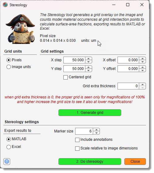
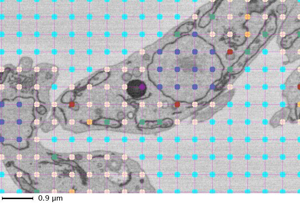
The Stereology tool overlays a regular grid on the image, identifies grid intersection points, and counts how many intersections fall on each model material. From these counts it calculates surface fractions and surface area estimates per material.

Launch via Ribbon → Tools → Stereology.

Workflow:

1. Segment objects of interest into a Model layer
2. Generate a grid (stored in the Mask layer) with 1. Generate grid
3. Run the analysis with 2. Do stereology

Grid units panel¶

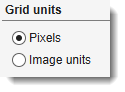Selects the unit system for all grid size and offset values.

• Pixels — all grid values are in pixels (default)
• Image units — all grid values are in the physical units defined in Dataset → Parameters (e.g., µm)

Grid settings panel¶

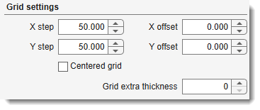
Defines the geometry of the grid. - X step — horizontal distance between grid lines (default 50 pixels). - Y step — vertical distance between grid lines (default 50 pixels).

• Centered grid — when checked, the grid is centred in the image (equal margins on all sides); when unchecked, the grid starts at the X offset / Y offset position.
• X offset — horizontal offset of the first grid line from the image edge (non-centred mode only).
• Y offset — vertical offset of the first grid line from the image edge (non-centred mode only).
• Grid extra thickness — additional dilation (in pixels) applied to each grid line via a cross-shaped structuring element. Use 0 for a single-pixel grid.

1. Generate grid — creates the grid and writes it to the Mask layer. If a mask already exists, you are asked to confirm before overwriting. The grid can be undone with Ctrl+Z.

Stereology settings panel¶

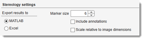
Controls how the analysis is performed and where results are exported.

Export results to (radio buttons):

• MATLAB — after analysis, prompts for a workspace variable name and assigns the results structure to it (default).
• Excel — saves results to a .xls file; prompts for a save path.

Options:

• Marker size — radius (in pixels) of the filled circle stamped on each grid intersection in the result model layer (default 6).
• Include annotations — also counts annotation labels from the Segmentation Panel → Annotations at each grid intersection. The counts are added to the exported structure under results.Annotations.
• Scale relative to image dimensions — when checked, intersection counts for boundary grid cells (cells partially outside the image) are scaled by the fraction of the cell area that lies inside the image. This corrects surface fraction estimates for grids that don't divide the image evenly.

2. Do stereology — runs the analysis. Requires:

• A Mask layer containing a grid (created by 1. Generate grid)
• A Model layer with labeled materials

Results are written back to the Model layer (intersection dots per material) and exported to MATLAB or Excel.

Exported results structure¶

The MATLAB results structure contains:

Back to MIB | User interface | Ribbon | Tools