Deep MIB - Predict Tab
Settings for efficient prediction (inference) and semantic segmentation model generation in Microscopy Image Browser.
How to start the prediction (inference) process
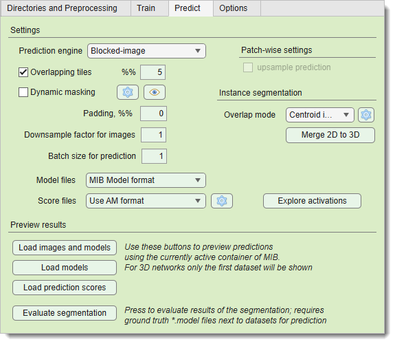
Prediction (inference) requires a pretrained network. if you lack one, train it first. pretrained networks can be loaded into Deep MIB for segmenting new datasets.
Steps to start prediction
- Select the pretrained network file in in the Network panel. This updates the Train panel with training settings. Alternatively, load a config file via Options tab → Config files → Load>
- Verify the prediction images directory in Directories and Preprocessing tab → Directory with images for prediction
- Confirm the output directory in Directories and Preprocessing tab → Directory with resulting images
- If needed (usually not), preprocess (convert) files:
- Set in the Directories and Preprocessing tab
- Click
- Switch to the Predict tab and press
Settings section
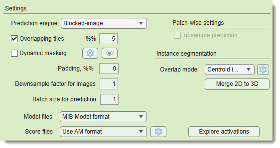
The Settings section configures prediction parameters.
: selects the tiling engine:
- Legacy used until MIB 2.83
- Blocked-image recommended for later versions (supports Dynamic masking and 2D Patch-wise)
: (for Padding: same) tiles the patches with overlap to minimize edge artefacts and improve segmentation. Define overlap percentage in
Overlapping vs non-overlapping mode
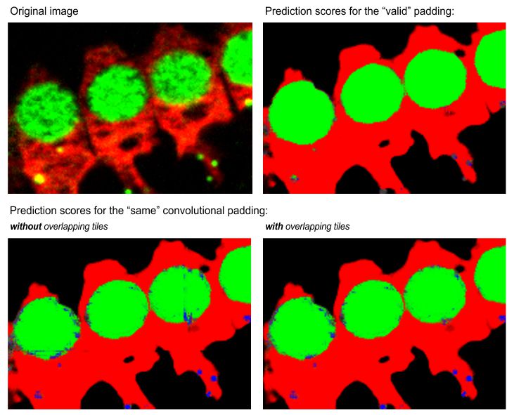
Same padding without overlap may show edge artifacts, reduced with overlapping mode.
: skips prediction on certain tiles using on-the-fly masking, configured via the  button
previews masking on the current Image View panel image
Dynamic masking settings and preview
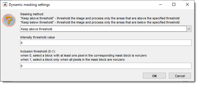
keeps blocks above or below the
sets the intensity threshold for prediction
fraction of pixels above/below threshold to keep a tile
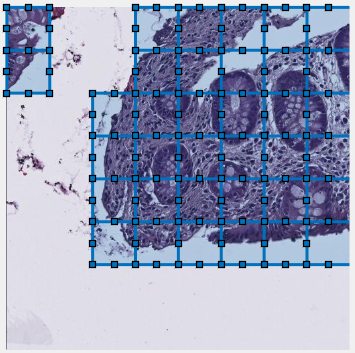
Masking preview
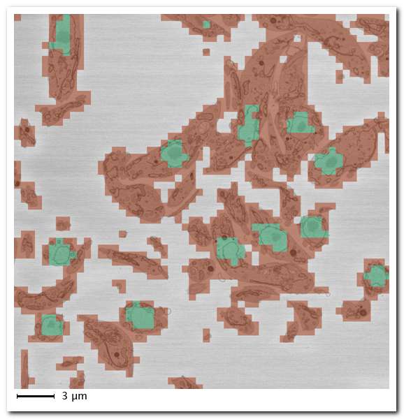
Example of patch-wise segmentation with dynamic masking
- Green: predicted nuclei
- Red: predicted background
- Uncolored: skipped patches
pads images symmetrically to reduce edge artifacts
downsamples prediction images to match training
(if applicable), upsampling results to original size and in case of networks with 2 classes are also smoothed
sets the number of patches processed by GPU simultaneously, limited by GPU memory
selects output format for models (CSV for patch-wise)
list of available image formats for the model files
- MIB Model format:
.modelfiles, loadable in MIB or MATLAB (model = load('filename.model', '-mat');) - TIF compressed format: LZW-compressed TIF, pixels encode classes (1, 2, 3, etc.)
- TIF uncompressed format: uncompressed TIF, pixels encode classes
selects output format for prediction score maps, configured via the button
list of available image formats for the score files
- Do not generate skips score files for better performance
- Use AM format AmiraMesh, compatible with MIB, Fiji, or Amira
- Use Matlab non-compressed format
.mibImg, loadable in MIB or MATLAB (model = load('filename.mibImg', '-mat');) - Use Matlab compressed format compressed
.mibImg, loadable in MIB or MATLAB - Use Matlab non-compressed format (range 0-1)
.mibImgwith 0-1 range, MATLAB-only (model = load('filename.mat');)
- : (2D patch-wise only) upsamples downsampled patch-wise predictions to match original image size
Instance segmentation subpanel
Settings of the Instance segmentation subpanel are only available for the 2D Instance workflow.
: selects how object instances are stitched across tiles during prediction:
- Centroid in core — each object is emitted by the tile owning its centroid; the tile overlap must exceed the largest object
- IoU merge — detections of neighbouring tiles are merged when their masks agree in the overlap band; works for objects larger than the overlap
An image that is no larger than the network input patch is segmented in one piece, so the overlap mode and the tile overlap settings have no effect on it.
The button configures the stitching parameters:
- — minimal confidence score for a detected instance to be kept (both overlap modes); decrease to detect more (weaker) objects, increase to keep only confident detections (default:
0.5) - — (IoU merge only) merge detections of neighbouring tiles when the intersection-over-union of their masks within the shared overlap band exceeds this value; decrease when objects get split at tile seams, increase when distinct touching objects get merged (default:
0.5) - - (IoU merge only) additionally merge when the intersection over the smaller in-band mask area exceeds this value, catching a truncated fragment fully contained in the neighbouring tile's complete mask; applied only to fragments that are really cut by a tile edge (default:
0.8) - - (both overlap modes) after stitching, each index is split into its separate objects so that two isolated objects never share one index; components smaller than this are discarded as speckle, set to
0to keep every component (default:100)
stitches the predicted instance models in
3_Results/PredictionImages/ResultsModels into 3D instance models, linking objects that overlap
between neighbouring slices into 3D instances with a consistent index. The layout is detected
automatically: 2D models are the Z-slices of one stack (taken in alphabetical order as the
Z-order) and give a single merged model, while 3D models (predicted from z-stack images) are
each stitched independently into one merged model per file. A dialog asks for the stitching
settings, then for the destination and file format; the result can be saved as a single 3D file or
as a sequence of 2D files. See the
2D Instance workflow for details.
Explore activations
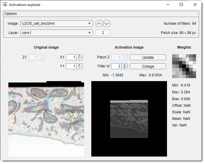
The Activations explorer evaluates network performance in detail. It is possible to see details of weights and activation images for all layers and filters.
- lists preprocessed prediction images. select one to load a patch matching the network’s input size. use arrows to navigate
- lists network layers. selecting a layer triggers prediction and activation image generation
- , , shifts the patch across the image. Update activations with
- adjusts Z within 3D network activation patches
- cycles through activation layers
- recalculates activations for the current patch
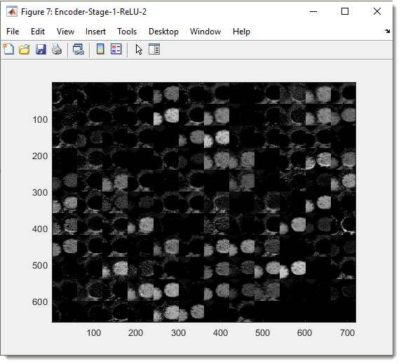
- creates a collage of current layer activations
Snapshot with the generated collage of activation images
Preview results section
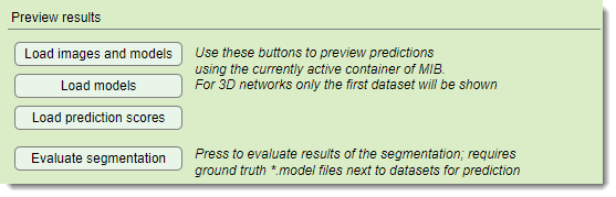
loads original images and segmentations
into MIB’s active buffer post-prediction
loads segmentations over the current MIB image. Requires that the image is already preloaded.
loads score images (probabilities) into the active buffer
calculates precision metrics if
ground truth labels exist in Labels under PredictionImages. Material names must match training data
Details of the Evaluate segmentation operation
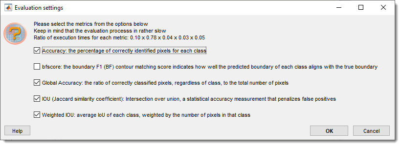
Select metrics to compute:
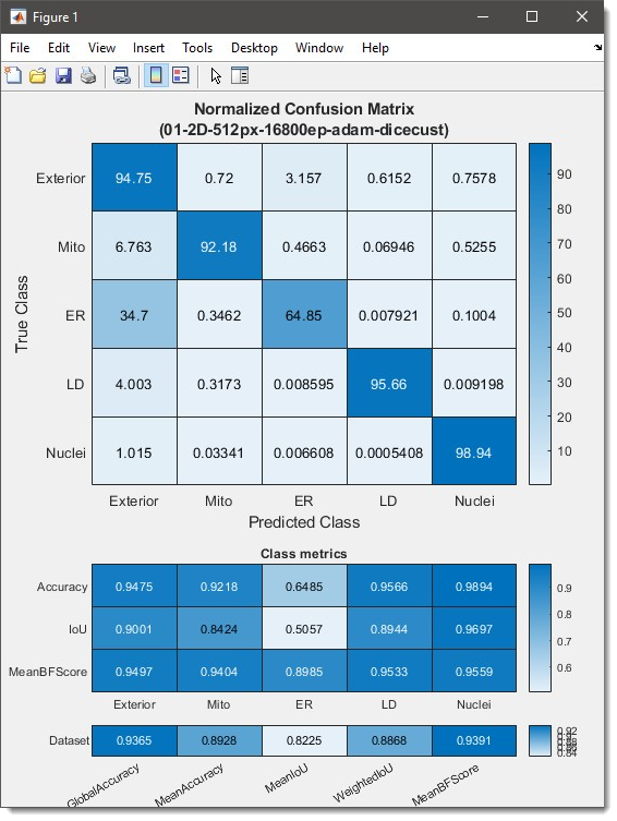
Results show a confusion matrix (0-100 scale), class metrics (Accuracy, IoU, MeanBFScore), and global metrics:
Additional metrics (label occurrence, Sørensen-Dice coefficient) are available via the dropdown:
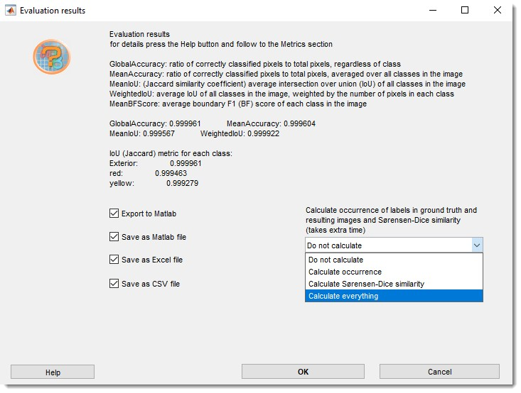
Export results to MATLAB, Excel, or CSV in 3_Results/PredictionImages/ResultsModels
(see Directories and Preprocessing). Details of the evaluation procedure are in
MATLAB evaluatesemanticsegmentation