Model Ribbon Tab¶

Overview¶

Actions that can be applied to the Labels layer. The Labels layer is one of three main segmentation layers (Labels, Selection, Mask) which can be used in combination with other layers. See more about segmentation layers in the Data layers section.

Convert Section¶

Convert type¶

Model Ribbon Tab

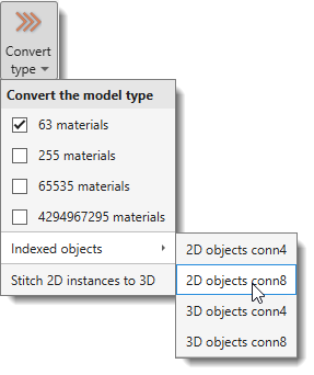
Convert the model to a different type; the current type is indicated in the ribbon. The Labels, Selection and Mask layers are backed up before the conversion, so it can be undone with Ctrl+Z, which brings back the previous model type together with its materials and colors.

Types of models in MIB

63 materials (default): Stores Labels, Selection, and Mask layers in a single memory container, reducing memory requirements with some performance costs and limiting materials to 63.
255 materials: Allows up to 255 materials, requiring additional memory for Selection and Mask layers (doubles memory usage).
65535 materials: Allows up to 65535 materials, requiring ~1.25× more memory than 255 materials. The Segmentation panel appearance changes in this mode.
Short demonstration
4294967295 materials: Allows up to 4294967295 materials, requiring twice the memory of 65535 materials.

Indexed objects

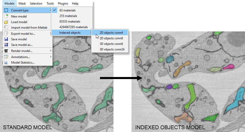
Detects objects in all materials and generates a new model where each object has a unique index:

2D objects conn4: 2D connected objects, 4-connectivity.
2D objects conn8: 2D connected objects, 8-connectivity.
3D objects conn4: 3D connected objects, 4-connectivity.
3D objects conn8: 3D connected objects, 8-connectivity.

Example: standard model converted to indexed objects

How to work with models having more than 255 materials

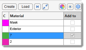Materials should be named with numbers representing the current working material index (e.g., 11555 means that when selection is added to the model, it will be assigned to index 11555).

Select materials by:

Right-clicking the segmentation table and choosing Rename... or by pressing F2
Hovering over an object in the Image View panel and pressing Ctrl+F.

The + (Add a new material to the model) button of the Segmentation panel scans the model for the highest index currently in use and switches the working material to the next free one. It does not create anything until you paint, so pressing it twice in a row offers the same index.

Stitch 2D instances to 3D

Links a stack of independently segmented 2D instances into consistent 3D objects. Unlike the Indexed objects options above - which turn a semantic model into indexed objects by connected-component analysis - this expects a model whose slices are already per-slice 2D instances, typically the raw output of a 2D instance-segmentation prediction where the same object carries a different index on each slice.

Objects that overlap between neighbouring slices are merged into a single 3D instance with one index through the whole stack. A settings dialog decides what counts as an overlap and how the leftovers are cleaned up.

See details

Import Section¶

New model¶

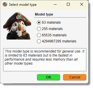
Create a new model and select the appropriate type

Allocates space for a new model. Use this to start a new model or delete the existing one.
Alternatively, use the New button in the Segmentation Panel.

For model types see Convert type above.

Load model¶

Loads a model from disk. By default, MIB reads models in MATLAB format (.model), but other formats are supported.

Compatible model formats

AM, Amira Mesh: Amira Mesh label field for models from Amira.
NRRD, Nearly Raw Raster Data: Compatible with 3D Slicer.
MRC, Medical Research Council format: Compatible with IMOD. Can load multiple MRC files, each encoding an object, and merge them into a single model.
PNG, PNG format: Saves models as 2D slices in Portable Network Graphic format.
TIF, TIF format: Saves models as 2D slices or 3D volumes in Tag Image File format.

Tip

Almost any standard image format can be loaded as a model using the All files (.) filter in the Open model dialog.

Alternatively, use the Load button in the Segmentation Panel.

Note

Models can also be opened by drag-and-dropping model files into the Image Document.

Note

When a loaded model carries no material names of its own (format-dependent - some formats, like Zarr, may or may not embed names), materials are auto-named mat1, mat2, … For models with more than 255 materials, plain numeric names are used instead, since the number is the material index - see the note on working with such models in Convert type above.

Import¶

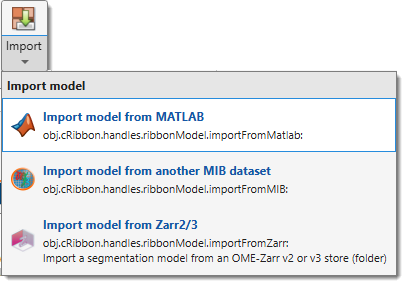
Import model from the main MATLAB workspace

Imports a model from an external source.

The Import dropdown contains:

Import model from MATLAB¶

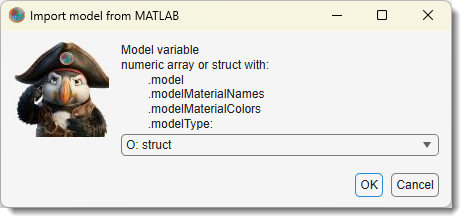
Imports a model from the main MATLAB workspace. Provide a variable name with a matrix matching the dataset dimensions [height, width, depth] of uint8 class, or a structure with the fields below.

Fields of the MIB model structure

.model: Matrix [height, width, depth, time] of uint8 class.
.modelMaterialNames (optional): Cell array with material names.
.modelMaterialColors (optional): Matrix with colors (0-1) [materialIndex, R G B].
.labelText (optional): Cell array with annotation labels.
.labelPosition (optional): Matrix with annotation positions [annotationIndex, x y z].

Import model from another MIB dataset¶

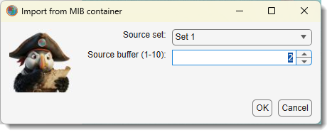
Copies the model from another currently open MIB dataset into the active dataset.

Import model from Zarr⅔¶

Imports a segmentation model from an OME-Zarr v2 or v3 store. A Zarr store is a folder (not a single file), so this option opens a folder browser instead of the file dialog used by Load model and the other Import options above.

Both Zarr v3 (.zarr3) and Zarr v2 (.zarr2) are read by the native zarr-matlab library, with no Python required. See Preferences → Zarr library if you want to read them through zarr-python instead.

Material names and colours

Material names/colours are resolved from the store's metadata, in this order:

MIB's own mibMaterials attribute (the same one written by Export model to Zarr3).
The OME-NGFF image-label convention (colors / properties).
If neither is present, materials are auto-named mat1, mat2, … with random colours.

Note

For a BigData dataset, importing a Zarr model attaches the store by reference instead of loading it into memory (see BigData datasets).

Whether it is editable depends on who wrote the store, not on its zarr format. A store MIB created itself - in either format - is a fully editable, disk-backed model, because it holds MIB's packed bytes and is stamped with a marker attribute that says so.

A store written by another tool is attached read-only: its values are that tool's own label indices, laid out in its own axis order, and writing MIB's packed bytes back into it would corrupt them. You can view and browse such a model at any zoom level. To segment on the same dataset, create a new model instead - MIB writes its own store and leaves the imported one untouched.

Export Section¶

Save or export the model to files and external programs.

Export¶

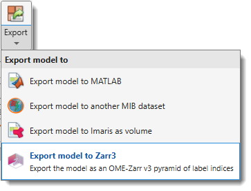
Exports the model to an external destination. The Export dropdown contains:

Export model to MATLAB: Exports to the main MATLAB workspace as a structure (see Import model from MATLAB for structure fields). Can be re-imported using Import model from MATLAB.
Export model to another MIB dataset: Copies the model into another currently open MIB dataset.
Export model to Imaris as volume: Exports to Imaris if available. See System Requirements for details.

Export model to Zarr3: Export the model as a chunked, pyramidal OME-Zarr v3 store (.zarr3) - material names and colours are preserved; reopenable in MIB as a BigData model and by external OME-Zarr-compatible tools

Export to Zarr3 - dialog settings (model)

A settings dialog appears after choosing the output path. Defaults are adapted to the open dataset dimensions (WSI vs. 3-D volumetric).

Setting	Description
Pyramid levels (0 = auto)	`0` = auto: starts at full resolution, adds levels while min(Y, X) / 2 ≥ 256 px, up to 8 levels. Enter 1-12 to force a fixed count.
Chunk size [Y, X, Z]	Zarr chunk dimensions in pixels.
Shard X-factors [Y, X, Z]	Chunks to bundle per axis into one shard file (0 on any axis = no sharding).
Compression	`zstd` (default), `gzip`, `none`.
Downsampling method	See table below. The downsampling strategy is always XY only for models - Z is never averaged, since that would mix material indices across boundaries.

Downsampling method

Method	Speed	When to use
nearest (default)	fast	Most models - picks the nearest source pixel; exact label integers are preserved.
mode	slow	Fine structures, thin boundaries - picks the dominant label in each output block (majority vote). More semantically accurate; ~4-8× slower than nearest.

Smart defaults (computed from the open dataset)

Dataset type	Chunk [Y, X, Z]	Shard X-factors
WSI (Z ≤ 2 slices or max(Y, X) ≥ 8 000 px)	512 × 512 × 1	4 × 4 × 1
3-D, near-isotropic (vxZ < 2 × vxXY)	128 × 128 × 64	4 × 4 × 1
3-D, anisotropic (vxZ ≥ 2 × vxXY)	256 × 256 × 16	4 × 4 × 1

Save model¶

Saves the model to a file in MATLAB format without prompting for a filename.

Filename resolution

Default template: Labels_NAME_OF_THE_DATASET.model.
Otherwise, the filename from the last Save model as... operation.
Otherwise, the filename assigned when the model was loaded.

Info

Can also be saved using the Save model button in the Quick Access Bar.

Save model as...¶

Prompts for a filename and format to save the model.

Available formats

Exporting a pyramid level (BigData models)

For a disk-backed BigData model, the Save model as... dialog adds a Pyramid level selector (s0 = full resolution … sN = coarsest). The chosen level is streamed to disk one slice at a time, so the full model is never loaded into memory. Per-slice streaming is available for TIFF, the native MODEL (*.model), HDF5 and OME-Zarr v3; other formats write the selected level as a whole.

The same selector appears for a segmentation imported from a URL as an overlay, with one difference: the levels listed are the segmentation's own, which start coarser than the image, so each is labelled with how much coarser than the image voxel it is. There is no full-resolution level to default to, which is why the level has to be chosen.

BigData models - format compatibility & memory use

All formats above can save a BigData model at the chosen pyramid level. They differ only in how much memory the write needs:

Format	BigData	Memory-optimized (streamed slice-by-slice)
MODEL (`.model`) - native*	✅	✅ disk-backed matfile
TIF	✅	✅
HDF5 (`*.h5`)	✅	✅
OME-Zarr v3 (`*.zarr3`)	✅	✅
AM, MAT, MOD, MRC, NRRD, PNG, STL, mibCat	✅	❌ selected level is gathered whole before writing

Use the Pyramid level dropdown to bound memory - a coarse level is small. The memory-optimized formats never hold even one full level in memory, so prefer them when exporting the full-resolution level (s0) of a large model.

Model tools Section¶

Materials¶

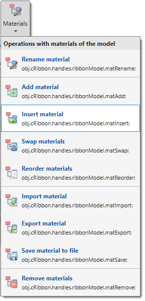
Operations for model materials, also available by right-clicking the Segmentation table.

Materials menu demo

The Materials dropdown contains:

Rename material: Rename the selected material.
Add material: Add a new material to the bottom of the list.
Insert material: Insert a material at a specified position, shifting others down.
Swap materials: Swap positions of two materials.
Reorder materials: Reorder materials with a new sequence.
Import material: Import selected materials (names, colours, and voxels) from a saved model file into the current model. You choose which materials to import; they are appended as new materials and their voxels overwrite the current ones where they overlap. For disk-backed BigData models the source is matched to the closest pyramid level and resized to fit.
Export material: Export the selected material to MATLAB or Imaris.
Save material to file: Save the selected material to a file.
Remove materials: Remove selected material(s) from the model.

List of annotations¶

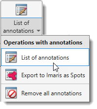
Operations for the Annotations layer.

Demonstration

The List of annotations dropdown contains:

List of annotations: opens the annotations window (see Segmentation Tools).
Export to Imaris as Spots: exports annotations as Spots in Imaris (export the dataset first).
Remove all annotations: deletes all annotations in the model.

Instance editor¶

Corrects individual objects of an instance model by hand: splitting one object into two, merging several into one, bridging a gap between two halves of the same object, and deleting false detections. Objects are picked from a list, by clicking them in the image, or by drawing over them in the Selection layer.

It is the proofreading step after Stitch 2D instances to 3D, which leaves errors that no threshold can remove. Requires an instance model (65535 or 4294967295 materials), where every object has its own index.

See Instance editor for details.

Render¶

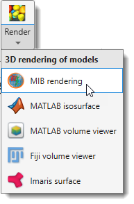
Renders segmented models using various methods. The Render dropdown contains:

MIB rendering¶

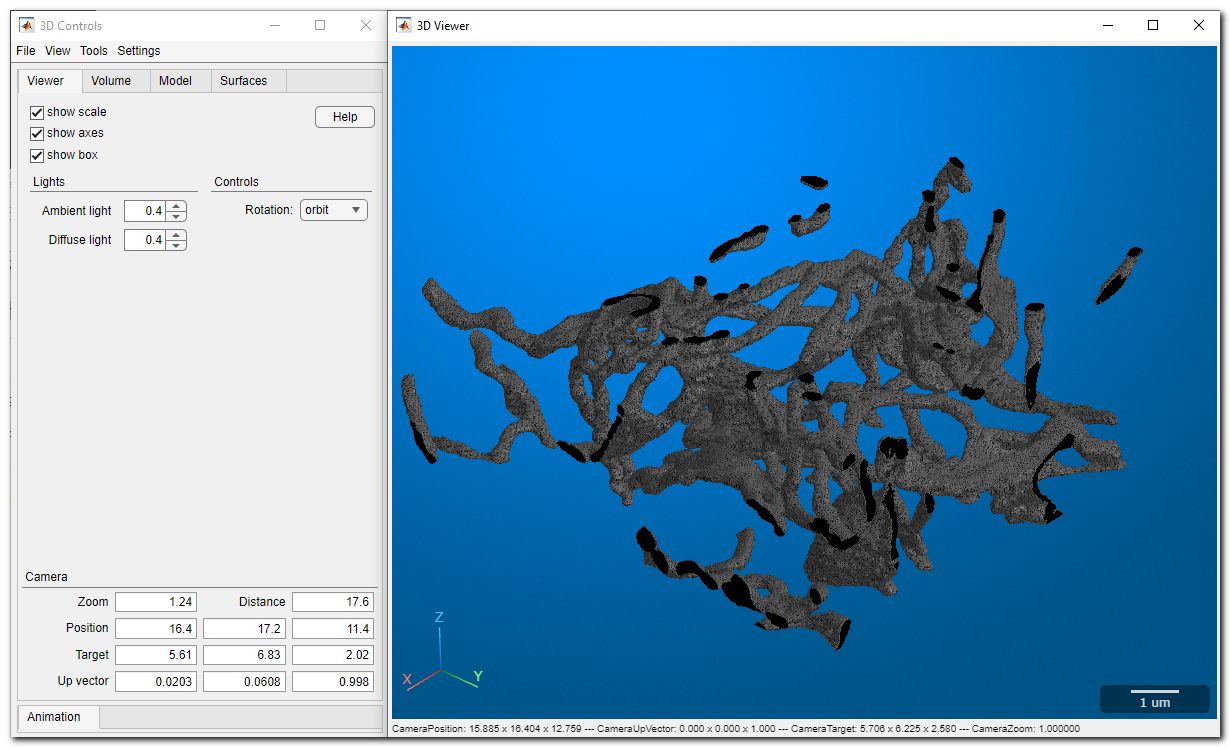
Materials can be visualized in MIB with hardware-accelerated volume rendering (MIB 2.5+, MATLAB R2018b+). Datasets can be downsampled. Snapshots and animations are supported.
See more: MIB 3D Viewer

Introduction to updated 3D viewer
Original version of 3D viewer

MATLAB isosurface¶

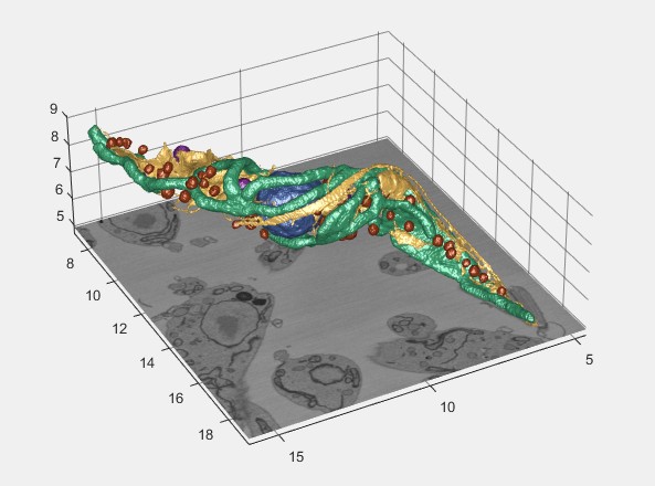
Uses MATLAB to generate and visualize isosurfaces with a modified view3d function by Torsten Vogel.

Demonstrations

Controls

Double to restore the original view.
other controls available from a toolbar menu in the upper-right corner and via

MATLAB volume viewer¶

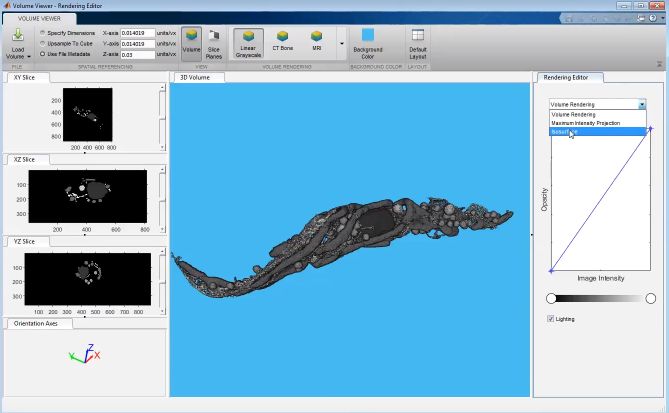
Renders the model using MATLAB's Volume Viewer (R2017b+). In R2019b+, materials can be displayed alongside the volume.

only for the MATLAB version of MIB

Demonstrations

Fiji volume viewer¶

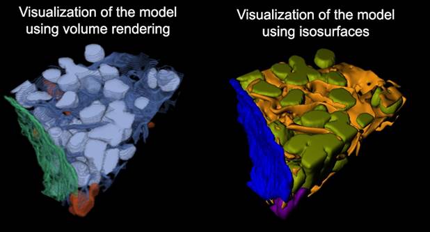
Uses Fiji 3D Viewer for volume visualization.
Requires Fiji installation (see System Requirements).

Demonstration

Imaris surface¶

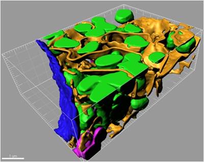
Renders the model in Imaris. Requires Imaris and ImarisXT (see System Requirements).

Demonstrations

The rendered material is specified in the Materials list of the Segmentation Panel.

Quantification Section¶

Quantify¶

Gets quantification statistics for the selected material, usable to filter the model by object properties.

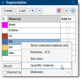
Accessible also via Segmentation Panel → Materials List → Right-click → Quantify material...

See Mask and Model Quantification for details.

Back to MIB | User interface | Ribbon