Dataset types
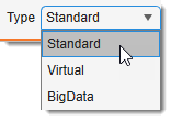
Every buffer in MIB stores its dataset in one of three types, chosen with the selector at the bottom of the Datasets panel. The type controls how the pixels are held - entirely in RAM, streamed from disk for browsing, or streamed from disk and segmentable - and therefore which datasets you can open and what you can do with them.
When a real dataset is open, switching the type shows a confirmation first (the current dataset is closed or converted); switching the type of an empty/placeholder buffer happens silently. Choosing BigData while a dataset is open offers Convert current (write the open image to an OME-Zarr v3 pyramid on disk and reopen it in BigData mode) or New (start an empty BigData placeholder).
| Type | In memory? | Editable model? | Typical use |
|---|---|---|---|
| Standard | whole dataset in RAM | ✅ full | small-medium datasets |
| Virtual | read on demand | ❌ browse-only | quickly browse datasets too large for RAM |
| BigData | read on demand, pyramidal | ✅ disk-backed model | segment datasets far larger than RAM |
Cold vs. warm start - Bio-Formats / WSI files (CZI, NDPI, …)
Virtual and BigData datasets that stream from a Bio-Formats / whole-slide file pay a one-time cold-start cost the first time a given file is opened: Bio-Formats must scan the file's internal tile/metadata directory before any pixels can be shown. This ranges from a second or two for a small file to several minutes for a very large multi-gigabyte image, and is far slower when the file lives on a network drive rather than a local disk. (By contrast, the pixel reads after opening are cheap - a zoomed-out view reads only a small pyramid level.)
MIB caches this parse in a small Bio-Formats Memoizer index (a .bfmemo file kept in
Bioformats Memoizer temporary directory that can be specified from MIB Preferences.
, so every later open of the same file is near-instant - even after
restarting MIB. Renaming/moving the file, or replacing it with a newer copy, invalidates the
cache and triggers one more cold start.
Datasets already stored as an OME-Zarr v3 pyramid have no cold-start cost (a chunked store needs no directory scan). For the fastest first open of a Bio-Formats / WSI file, keep it on a local disk rather than a network share; opening it once also warms the cache for later sessions.
Standard
The entire dataset is loaded into RAM. This is the default and the most capable mode.
- Best performance - all pixels are immediately in memory.
- All tools, filters, processing and export formats are available.
- Full multi-step Undo/Redo.
- The dataset (and its model/mask/selection layers) must fit in RAM, with headroom for processing.
- Not suitable for datasets larger than available memory - use Virtual (to browse) or BigData (to browse and segment) instead.
Virtual
Pixels are read from disk on demand (e.g. an OME-Zarr v3 pyramid, HDF5, or a BioFormats-backed file), so only the currently viewed region is held in memory.
- Open and browse datasets far larger than RAM with a small memory footprint.
- Supports more on-disk formats than BigData (anything the virtual readers can stream).
- Browse-only - segmentation layers (Selection, Mask, Model) and most pixel-editing/processing tools are disabled; Undo is not kept for these layers.
- Slower per access than Standard (each view reads from disk).
- To segment a large dataset instead of just viewing it, use BigData.
BigData
For datasets too large to fit in RAM that you also want to segment. The image is a pyramidal source read on demand (zoom selects the matching resolution level; pan reads only the visible region), and the segmentation model is a disk-backed, pyramidal 63-class store that mirrors the image pyramid. Edits are written straight to disk and propagated across levels, so a model can be far larger than memory and survives across sessions.
Two kinds of image can serve as that source:
- an OME-Zarr v3 store, opened directly;
- any pyramidal file that Bio-Formats or OpenSlide can read - the whole-slide formats such as SVS, NDPI, CZI and their relatives - streamed straight from the vendor file, with no conversion step.
Whichever the image is, the model is always written as an OME-Zarr v3 store beside it, named
Labels_<name of the image>.zarr3.
- Segment datasets much larger than RAM - only the visible region/level is ever in memory.
- The model is saved live to disk (an OME-Zarr v3 group next to the image) and reloads across sessions; material names and colours are preserved.
- Smooth zoom/pan and orientation switching (XY / ZX / ZY) by reading the appropriate pyramid level.
- Export any pyramid level to standard formats, streamed slice-by-slice for the memory-optimized formats (see Save Image As and Save model as...).
- Selectable Zarr backend (native
zarrMexorzarr-python); define in Preferences->Input / Output - 3D volume rendering - the → button on the Home ribbon now supports BigData: pick a pyramid level to render in 3D (a memory estimate is shown for each level), and optionally enable the live-update checkbox so the overlay refreshes automatically as you segment in the main window.
- The source must be pyramidal. An OME-Zarr v3 store or a pyramidal Bio-Formats / OpenSlide file opens as BigData as it stands, but a format with only one resolution level (a plain TIFF, an HDF5 volume, a folder of slices) has no levels to stream and must first be converted - switch the type dropdown to BigData → Convert current, or use Ribbon → Home → Export → Export to Zarr3, or the Image converter plugin.
- Streaming from a vendor file pays the cold-start cost described above; an OME-Zarr v3 store does not. Converting a slide you will return to often therefore still pays off.
- Browse-only until a model exists - create a model (Segmentation panel → Create, or Ribbon → Model → New model, or load one) to enable segmentation.
- Up to 63 materials (packed model), and a single time point (time-series is not yet supported).
- The source image is read-only - you edit the model, not the image pixels. To change image pixels, convert the (cropped) region to Standard.
- A few tools are not available: Object Picker, Black-and-White Thresholding, and SAM's Automatic everything. Each segmentation tool page states its BigData support.
Getting into BigData mode
Set the Dataset type dropdown to BigData before opening, and a .zarr3 store or a
pyramidal whole-slide file opens straight into it. To move a dataset that is already open, switch
the same dropdown to BigData and choose Convert current, which writes an OME-Zarr v3 pyramid
to disk and reopens it.
Remote stores
A Virtual or BigData dataset does not have to sit on your disk. MIB can open an OME-Zarr container from a public cloud bucket over the network - see Import from URL / Zarr - and only the tiles you actually look at are transferred.
Three things are worth knowing before you rely on it:
- The model store is always local. When you create a model on a remote BigData dataset, MIB asks where to put it and writes an OME-Zarr pyramid to your own disk. The remote image is never written to.
- No Python is required, in either zarr format. The bundled native engine fetches remote v2
and v3 stores with HTTP range requests. Python is only used if you deliberately select the
pythonengine in Preferences → Zarr library, and that engine does needaiohttpandrequestsfor remote access. - Decoded chunks are held in a memory cache, so revisiting a slice or panning back over ground you have already seen costs nothing. Its size is set by Preferences → Chunk cache. Reaching genuinely new tiles is still a network round trip, so the pyramid is what keeps zoomed-out browsing responsive; working at full resolution on a remote volume remains slow by nature.
A published container often also holds small, densely annotated ground-truth crops. Selecting one opens it as a Standard dataset in its own right: MIB cuts the matching region out of the parent image, loads that, and puts the selected annotation classes on it as a model - see Label crops. Painting such a crop onto the full parent volume as an overlay is a different thing, and is not supported.
How BigData works
This section explains the machinery behind BigData segmentation - useful for understanding why editing stays fast on a multi-gigapixel slide and what the Save model options do.
The image and model pyramids
A BigData image is a pyramid: the same picture stored at several resolutions
(s0 = full resolution, s1 = half/quarter, … sN = coarsest thumbnail), each split into small
chunks on disk. When you zoom, MIB picks the pyramid level whose scale is nearest to the
current magnification; when you pan, it reads only the chunks under the viewport. Nothing else is
loaded, so memory use stays tied to the size of the window on screen, not the size of the slide.
At a magnification that falls between two levels, the block read from the chosen level is then resampled to the exact scale on screen. Because the nearest level is taken, this goes either way: you may be seeing a finer level scaled down, or a coarser level scaled up, whichever level's scale was closer.
Which level wins, exactly
Each level carries a scale factor relative to full resolution (s0 = 1, s1 = 2, s2 = 4, …),
and MIB takes the level whose factor differs least from the current magnification. A tie goes to
the finer level.
With levels at 1x, 2x and 4x:
| Magnification | Level used | What happens to it |
|---|---|---|
| 2x | s1 (2x) |
used as read, no resampling |
| 3x | s1 (2x) |
tie with s2, so the finer one is scaled down |
| 3.5x | s2 (4x) |
nearer than s1, so it is scaled up |
The resampling is nearest-neighbour, which is fast and never invents intermediate intensities; upscaling a coarser level therefore looks blocky rather than smooth. Zooming a little further in crosses to the finer level and the detail returns.
This applies to the display path only. Tools that ask for a specific pyramid level (export, 3D rendering) read that level directly, with no resampling.
The model (your segmentation) is stored the same way: a parallel pyramid of the same levels, packed so each voxel holds the material index plus the mask and selection bits. It lives in an OME-Zarr v3 group next to the image and is written live as you segment - there is no separate "load the whole model into RAM" step.
Edits are written at the zoom you draw - plus coarser
When you paint at, say, 16% zoom, the stroke is written to that pyramid level and every coarser level immediately (a coarser level is small, so downsampling the edited patch into it is cheap). The finer levels (higher resolution than where you drew) are not written right away - they are marked as needing an update and reconstructed later. This is what keeps a brush stroke cheap regardless of zoom or slide size: the cost scales with the edit, not with the whole image.
Finer levels are rebuilt on demand (and cached)
When you zoom in to a level finer than where an edit was made, MIB reconstructs that region for the finer level by up-sampling from the level that holds the data, writes it down, and caches it - so the next view of the same area is a direct read with no recomputation. An optional, label-aware smoothing (Preferences → Input/Output → Zarr → Smoothing) removes the blocky stair-steps that plain up-sampling would produce at the finer grid.
The level map and its sidecar file
To know, for every region, which level currently holds the real data, MIB keeps a small level map. It records per tile the finest materialized level, so reads know whether they can go straight to disk or must reconstruct first. Two consequences follow:
- Selection-aware operations are fast. Assigning the selection to a material and the other shortcuts ( / / ) and clearing it () work only inside the selection's tracked footprint instead of scanning the whole slide.
- The map is persisted as a sidecar file next to the model store, named
<model-name>.levelmap(for exampleLabels_CMU-1.levelmap). It is written when you close the model and when you press Save model (see below). It does not exist mid-session until you save or close.
Why a loaded model is always precise
A model on disk is treated as precise at every level unless the sidecar explicitly says some tiles still have deferred (not-yet-written) finer levels. So an imported / externally-created model - where the whole pyramid was written properly - loads at full detail; deferral is purely a within-a-session optimisation, and that state lives in the sidecar.
Saving a BigData model
Pixel edits are already on disk the moment you draw them; the only volatile state is the in-memory level map. Pressing on the Model ribbon therefore offers two choices:
| Choice | What it does | Speed |
|---|---|---|
| Finalize & save | Materializes every resolution level from the level map, so the on-disk model is consistent at all zooms - required for export and for opening the store in external readers. | slower on a large slide |
| Save sidecar | Writes only the small level-map file. A fast crash-safety checkpoint: because edits are already on disk, persisting the level map is enough for a reopen to restore the model precisely (rebuilding deferred finer levels on demand) without re-materializing. | fast |
The sidecar file is kept after Finalize - this is expected
After Finalize & save, the .levelmap sidecar file is not deleted: it is updated to record
that every level is now fully materialized. On the next open MIB reads that record and knows the
model is complete. Without the sidecar, MIB would reach the same conclusion via a fallback - but
keeping it makes the distinction between a fully-materialized model and one with deferred levels
explicit and reliable. You can safely ignore the sidecar file - do not delete it, as it is the
only durable marker that the model is consistent at all zooms.
Protect against a crash
During a long session, use Save model → Save sidecar periodically. If MIB then closes unexpectedly, reopening the model reads the sidecar and restores everything you drew - at every zoom - without the cost of full finalization. Run Finalize & save once at the end (or before exporting) to write every level to disk.
Efficiency in one line
Edit cost scales with the size of the edit, not the size of the slide: small footprints are read, merged, written and propagated; finer levels are deferred and rebuilt lazily; and the level map lets both reads and selection operations target exactly the region that changed.
Back to MIB | Getting Started